ml.doc (1.1): Learning from data
How does a computer learn from experience?
Over the last few weeks I’ve been working through MIT’s machine learning course (6.86x). The course’s emphasis on understanding the core concepts really makes you think about the data and whether a given algorithm is the right tool for the job. This approach would benefit those who are new to machine learning and looking to employ ML algorithms in their own work. On the other hand, the course itself requires some mathematical maturity (not to mention a bucketload of undergraduate algebra and calculus) which can make the material hard to digest. A little exposition in the right places would go a long way towards helping new practitioners use these new tools more effectively in their projects.
To address this thought bubble (and reinforce my own understanding), I’ve decided to write up some key ideas introduced in MITx 6.86x so as to make them more accessible to a general audience. Think of each writeup as being inspired by the MIT approach, but with some extra material in places to help absorb the ideas.
Table of Contents
The job of a classifier is to take some input data and figure out how to label it. Many successful applications of machine learning involve classification, ranging from recommender systems to spam and fraud detection to medical diagnosis. This writeup will be focused on classifiers that are both binary (i.e., two output label choices) and linear, where the label output is a linear function of the inputs.
Overview
A classifier $h$ is a function that maps an input feature vector $x$ to a discrete output label, $y = h(x)$. The function is discovered during a training period in which the classifier is exposed to data from a training set $S_{N}$, consisting of $N$ input examples and their labels,
$$S_{N} = \{ (x^{(i)}, y^{(i)}), i=1,…,N \}.$$
Imagine you want to build a classifier that can predict whether you will like a brunch dish, based on its ingredients. You might consider a six-item ingredient list:
- 🥔 potato
- 🥑 avocado
- 🍅 tomato
- 🥓 bacon
- 🍄 mushroom
- 🥫 baked beans
We will represent each brunch dish as a 6-dimensional feature vector, $x^{(i)} \in \{0, 1\}^6$, with $x^{(i)}_{k} = 1$ indicating the presence of the $k$-th ingredient in the $i$-th dish. The label $y^{(i)}=1$ is used to indicate that you like the $i$-th dish (and $y^{(i)}=-1$ to encode the opposite).
An example training set $S_5$ containing five example brunch dishes is shown below. Each component of $x$ (in other words, each ingredient $x_k$) is known as a feature.
| $i$ | dish | 🥔 $x^{(i)}_{1}$ | 🥑 $x^{(i)}_{2}$ | 🍅 $x^{(i)}_{3}$ | 🥓 $x^{(i)}_{4}$ | 🍄 $x^{(i)}_{5}$ | 🥫 $x^{(i)}_{6}$ | $y^{(i)}$ | |
|---|---|---|---|---|---|---|---|---|---|
| 1 | avocado sandwich | 0 | 1 | 0 | 0 | 1 | 0 | 1 | |
| 2 | huevos rancheros | 0 | 1 | 1 | 0 | 0 | 1 | 1 | |
| 3 | bacon and eggs | 0 | 0 | 0 | 1 | 0 | 0 | 1 | |
| 4 | english breakfast | 1 | 0 | 1 | 1 | 1 | 1 | -1 | |
| 5 | mushroom chowder | 0 | 0 | 0 | 1 | 1 | 0 | -1 |
After training our brunch classifier $h_{brunch}$ on the training set, it will learn how to map each input vector to its corresponding label. We could then use it to predict whether we would like something new, like breakfast burritos.
$$ \textrm{breakfast burrito} = \{🥔, 🥑, 🍅, 🥫\} $$ $$ h_{brunch}(\{🥔, 🥑, 🍅, 🥫\}) = h_{brunch}([1, 1, 1, 0, 0, 1]) = … $$
Measuring error
Classifiers learn from their mistakes with the help of an algorithm. With each example $(x^{(i)}, y^{(i)})$ considered during training, the algorithm checks to see whether the classifier maps the input to the right label. If $h(x^{(i)}) \neq y^{(i)}$, the classifier has made a mistake. We define the training error $E_N$ as the average rate of mistakes over the training set,
$$ E_N(h) = \frac{1}{N} \sum_{i=1}^{N} [\![ h(x^{(i)}) \neq y^{(i)} ]\!],$$
where $ [\![ \textrm{something} ]\!] = 1$ if the thing inside is true, and $0$ otherwise. For example, $ [\![ 2 = 9 ]\!] = 0$ and $ [\![ 2 < 9 ]\!] = 1$. If our brunch classifier gets three of the five training labels wrong, then $E_N(h_{brunch}) = \frac{3}{5}$.
Knowing the training error is important, but we are usually more interested in how the classifier would perform in the real world, on data it has not seen before. Since we cannot know how well $h$ would work for every possible feature vector, we settle for knowing the test error $E(h)$, which is computed in the same way as the training error, but with data that have been set aside for this purpose.
Sketching the goal
We have talked about the idea of training a classifier to learn from mistakes, but what does that look like? Let’s use some sketches to visualize it.
Imagine we are midway through training a linear classifier on a set of $N=5$ two-dimensional feature vectors, $x \in \mathbb{R}^2$ (Fig. 1). Their labels, $y \in \{-1, 1\}$ are indicated by the plus/minus symbols. There is also a black line, running through the feature space and dividing it into two halves. This represents our linear classifier.
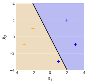
On the blue half of the feature space, vectors map to $h(x) = 1$, and on the orange half, $h(x) = -1$. We can see that all but one of the training examples have been mapped correctly. Since we have five examples, the training error $E_N(h) = 1/5$.
Not bad, but looking at the plot, you can see some room for improvement. If we just bump the line, this decision boundary a little bit, we can improve the classifier and achieve zero training error (Fig. 2).
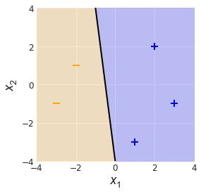
This, in a nutshell, is what training a classifier looks like. We start off with a function $h$ that is useless, but with each iteration of the algorithm, the decision boundary dividing each label region gets nudged and the function becomes slightly better at its job.
A mathematical translation
If you peer into the black box of a classifier and find out how it “learns”, you will be unsurprised to find some mathematics. What might surprise you is how little of it you need to know to more fully understand the general problem of classification. In this section we will motivate the use of linear algebra as a language to describe the problem at hand, using it to flesh out the ideas of the previous section.
The decision boundary
A binary classifier splits the feature space into two, using a decision boundary. Before we can update the classifier, it needs to be described in language that a training algorithm can understand. That is, we need to parameterize the decision boundary. Once we have this, the algorithm can update the decision boundary parameters to improve the classifier.
In general, the decision boundary is a function of the inputs. A linear classifier working in a $d$-dimensional feature space has a decision boundary that is a linear combination of the input features,
$$ x_1 \theta_1 + x_2 \theta_2 + … + x_d \theta_d + \theta_0 = x \cdot \theta + \theta_0 = 0 $$
where $\theta = [\theta_1, \theta_2, …, \theta_d] \in \mathbb{R}^d$ is a $d$-dimensional vector that determines the relative influence of each feature on the classification, and $\theta_0 \in \mathbb{R}$ is a scalar offset.
Note that the dot in $x \cdot \theta$ denotes the dot product of two vectors. Geometrically, this operation is defined by $\newcommand{\norm}[1]{|| #1 ||}$
$$ x \cdot \theta = \norm{x} \norm{\theta} \textrm{cos}\:\alpha, $$
where $\norm{x}$ is the norm of $x$ and $\alpha$ is the angle between the two vectors. If this looks completely foreign to you, it’s probably a good idea to stop here and learn the geometric implications of $x \cdot \theta$ before continuing. Make some sketches!
To get comfortable with what exactly $\theta$ means here, let’s scale the feature space back to two dimensions and play around with the simplest linear classifier: one whose decision boundary passes through the origin, i.e. $\theta_0 = 0$ (Fig. 3). In this case, the decision boundary takes the form of a line,
$$ x_1 \theta_1 + x_2 \theta_2 = x \cdot \theta = 0. $$
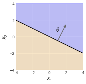
Let’s consider the geometry of our situation. This was not mentioned earlier, but by convention, $\theta = [\theta_1, \theta_2]$ is chosen such that it points towards the (blue) positively-labeled feature space, as indicated in the figure. Keep this in mind.
Now, any vector $x = [x_1, x_2]$ that lies exactly on the decision boundary satisfies $x \cdot \theta = 0$. That means $x$ and $\theta$ are perpendicular to each other, which makes sense. The other implication here is that the classifier has no idea what to do with these inputs: should it be unlucky enough to get them, it will map them to the label $y = h(x) = 0$.
How about some other options? Say we pick a positively-labeled vector $x = [-1.8, 2.6]$. Since the (smallest) angle between $x$ and $\theta$ is acute, we know that $x \cdot \theta > 0$ (Fig. 4, left). Now try a negatively-labeled one: $x = [-3.1, -1.7]$. This time, the dot product $x \cdot \theta < 0$ (Fig. 4, right). We are starting to see something useful here!
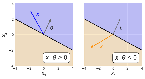
If we consider the general form of the classifier and add back the scalar offset, such that the decision boundary looks like $x \cdot \theta + \theta_0 = 0$, the key idea stays the same, e.g. if $x \cdot \theta + \theta_0 > 0$, the classifier assigns $x$ a positive label. In other words, $x$ gets mapped to the sign of the quantity $x \cdot \theta + \theta_0$.
The binary linear classifier
At last, we are ready for a proper definition. A binary linear classifier $h$ is a function that maps feature vectors $x$ to $h(x) \in \{-1, 0, 1\}$, where $$ h(x) = \textrm{sign}(\theta \cdot x + \theta_0).$$
The search for a good classifier now becomes a matter of finding values for the parameter vector $\theta$ and offset parameter $\theta_0,$ such that the classifier output or prediction $h(x^{(i)})$ is equal to $y^{(i)}$ for a decent proportion of the training set. We will talk about how we find these values very soon.
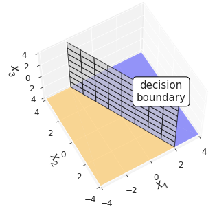
Although we have made use of two-dimensional examples, the same concepts hold in higher dimensions. In general, the decision boundary is a hyperplane of the feature space. All that fancy word means is that for a $d$-dimensional feature space, the decision boundary is an $(d-1)$-dimensional subset of that space. You have already seen that for a two dimensional feature space, i.e. $x \in \mathbb{R}^2$, the decision boundary is a line. If we move up another dimension and consider features $x \in \mathbb{R}^3$, the decision boundary becomes a plane, as shown below.
Linear separability
As it turns out, there is a price to pay for this level of simplicity: linear classifiers of this type are quite constrained. Consider the following two-dimensional dataset (Fig. 6). It is an illustration of XOR, the boolean operation that says you can have either one of these two things $(x_1=1 \textrm{ or } x_2=1)$, but not both $(x_1=1 \textrm{ and } x_2=1)$.
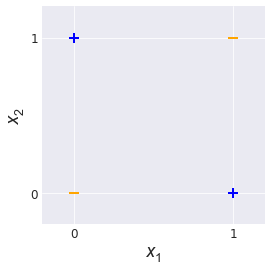
No matter how you slice it, there is no way to draw a line through these training examples to perfectly group them by label. This is an example of a dataset that is not linearly separable. More formally, the training dataset $S_N = \{(x^{(i)}, y^{(i)}), i=1,…, N\}$ is said to be linearly separable if there exists a parameter vector $\hat{\theta}$ and offset vector $\hat{\theta_0}$ such that for all training examples $i=1,…,N$,
$$ y^{(i)}(\hat{\theta} \cdot x + \hat{\theta_0}) > 0.$$
Take a moment to understand this expression. Imagine we have a pair of these special values $\hat{\theta}$ and $\hat{\theta_0}$ for some dataset. If we look at the above inequality for a positive example $x_+$, we know that $(\hat{\theta} \cdot x_+ + \hat{\theta_0})$ must be positive for it to hold, since $y_+=1$. Similarly, for a negative example $x_-$, the quantity $(\hat{\theta} \cdot x_- + \hat{\theta_0})$ must evaluate to a negative value.
What we can see here is that when $y^{(i)}(\theta \cdot x^{(i)} + \theta_0) > 0$, the label and classifier output for the $i$-th training example $x^{(i)}$ are in agreement. When this equality is not true, the prediction does not match the label and the classifier has made a mistake.
Teaching the classifier
It is finally time to talk about how a classifier learns from experience. Until now there have been many mentions of an “algorithm”, which is vaguely understood to be used for training the classifier. Here we will introduce the perceptron, a simple and elegant algorithm whose variants have been widely applied to solve all kinds of problems.
To train a classifier, an algorithm needs to recognize when the classifier makes a mistake. Recall that the training error for a linear classifier looks like this:
$$ E_N(h) = \frac{1}{N} \sum_{i=1}^{N} [\![ h(x^{(i)}) \neq y^{(i)} ]\!],$$
where $[\![ h(x^{(i)}) \neq y^{(i)} ]\!]$ equals one for a mistake, and zero otherwise. But thanks to our previous discussion, we know precisely how to express a mistake, i.e,
$$y^{(i)}(\theta \cdot x^{(i)} + \theta_0) \leq 0.$$
With that in mind, let’s take a stroll through the perceptron.
The perceptron
The perceptron algorithm takes a training set $S_N$ input, and outputs the classifier parameters $\theta$ and $\theta_0$. The general principle is to find a mistake and then update the parameters to fix the mistake. As long as the training data are linearly separable, doing this for long enough will eventually result in some parameters that do the job.
It is typical to initialize $\theta$ to a $d$-dimensional zero vector (where $d$ is the number of features) and $\theta_0$ to a scalar zero. For now we will ignore $\theta_0$ and focus on training a linear classifier whose decision boundary runs through the origin. We begin the proceedings with the following items:
theta, a $d$-element array of zeros,feature_matrix, a $d \times N$ feature matrix, with a training example on each row,labels, an array of $N$ labels for each training example.
An incomplete Python (Numpy) implementation of the algorithm looks like this:
def incomplete_perceptron(feature_matrix, labels):
    num_features, num_examples = feature_matrix.shape
    theta = np.zeros(num_features)

    for i in range(num_examples):
        x, y = feature_matrix[i, :], labels[i]
        # update theta when we have made a mistake
        if y * np.dot(theta, x) <= 0:
            theta = theta + y * x

    return theta
At the update step, the algorithm tests to see whether theta, the current iteration of the classifier computes the wrong training label. When that happens, $\theta$ is updated by adding $y^{(i)} x^{(i)}$ to it.
To see why that should help things, let’s consider the scenario after one update, where $\theta = y^{(i)}x^{(i)}.$ Now imagine if the classifier saw the same training example. If we plugged our updated $\theta$ value into the “mistake detector”, we would get
$$ y^{(i)} (\theta \cdot x^{(i)}) = y^{(i)} ((y^{(i)}x^{(i)}) \cdot x^{(i)}) = x^{(i)} \cdot x^{(i)} = \norm{x^{(i)}}^2$$
Now unless you happen to have a row of zeros inside your feature matrix, the squared norm of $x$ is always greater than zero, and so the mistake has been corrected. We can see that the algorithm has somehow improved the situation.
Number of iterations
As we go through the training examples, the parameter vector $\theta$ will change rapidly, sometimes cancelling out the effect of previous examples. It is for this reason that the dataset is typically iterated over multiple times, ideally until the algorithm no longer finds a mistake.
To complete the algorithm, we will introduce a new input $T$ that specifies how many times to loop through the dataset, and factor the offset parameter theta_0 into our computation. The last change to make is a practical one: it is tricky to check whether a numerical computation equals an exact value, like zero. To avoid numerical instabilities, we will instead use a tolerance parameter $\epsilon$, such that if some result $|r| < \epsilon$, then $r = 0$.
def perceptron(feature_matrix, labels, T=1, tolerance=1e-6):
    num_features, num_examples = feature_matrix.shape
    theta = np.zeros(num_features)
    theta_0 = 0

    for t in range(T):
        for i in range(num_examples):
            x, y = feature_matrix[i, :], labels[i]
            # update theta, theta_0 when we have made a mistake
            if y * (np.dot(theta, x) + theta_0) < tolerance:
                theta = theta + y * x
                theta_0 = theta_0 + y

    return theta, theta_0
The offset update
It is worth making a quick note about how the update for the offset parameter $\theta_0$ comes about. Consider a dataset that has been “extended”, such that $\theta_{ext} = [\theta, \theta_0]$ and $x_{ext} = [x, 1],$ where $x \in S_N$. If we want to update $\theta_{ext}$ using our extended training data, we use the same update rule as before,
$$\begin{align*}
\theta_{ext} &= \theta_{ext} + y^{(i)} x_{ext}^{(i)} \\
\end{align*}
$$
Expanding this out reveals the update for both parameters:
$$\begin{align*}
\begin{bmatrix}
\theta\\
\theta_0
\end{bmatrix}
&=
\begin{bmatrix}
\theta\\
\theta_0
\end{bmatrix}
\end{align*} + y^{(i)}
\begin{bmatrix}
x^{(i)}\\
1
\end{bmatrix}
$$
In other words, handling the extra offset parameter $\theta_0$ is just a matter of considering slightly different training examples.
Summary
Over the course of this writeup we have peeked behind the curtain and seen that machine learning, for all the hype and buzz, is not something overly mysterious. At heart, machine learning is the practice of identifying patterns in data using some kind of model, with the “learning” achieved through improving the model parameters.