Table of Contents

Allowing room for error

While the perceptron algorithm is easy to understand, the fact that it only works for linearly separable data really limits its application. Data collected in the real world are often measured with some error. They are noisy. Sometimes training examples can be accidentally mislabeled. There are many good reasons for an algorithm to allow some room for error and not let “the perfect be the enemy of the good”.

Let’s take a look at two different linear classifiers (Fig. 1). On the left we have a decision boundary that is extremely close to one of the training examples. The two dashed lines on either side are margin boundaries that expand until one of them hits a training example.

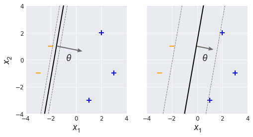
If you were to choose which classifier you would prefer, you would probably choose the one on the right, the one with a large margin. You can see that if the $(x_1, x_2)$ coordinates had more jitter, the classifier on the left might misclassify the negative training example sitting on the negative margin boundary. With all else being equal, we would prefer to use large margin classifiers that are more tolerant of natural variation.

To incorporate the idea of margins into our classification algorithms, we will formulate learning as an optimization problem that strikes a balance between two competing goals, the first of these being to achieve large classifier margins.

Margin boundaries

As seen earlier, linear margin boundaries are lines that sit on either side of the decision boundary, one for each label region in the feature space. Since the margins are parallel to the decision boundary $(\theta \cdot x + \theta_0 = 0),$ the margins take the form $\newcommand{\norm}[1]{|| #1 ||}$

$$ \theta \cdot x + \theta_0 = d.$$

The positive margin boundary, residing within the positive feature space region, is defined as $\theta \cdot x + \theta_0 = 1$ while the negative decision boundary on the other side is defined as $\theta \cdot x + \theta_0 = -1$. (Fig. 2).

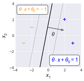
We can get a sense for how to control the width of the margins by considering the dynamics of $f(x) = \theta \cdot x + \theta_0$. As we move away from the decision boundary and towards the positive margin boundary, $f(x)$ increases at a rate proportional to $\norm{\theta}$, the magnitude of $\theta$. If we want to speed up how quickly we arrive at $f(x) = 1$ (and in doing so reduce the margin) we need to use larger values of $\norm{\theta}$.

Earlier, I mentioned that our optimization process has two competing priorities, one of which is to use large margins. The other priority seems quite natural: to achieve the highest possible classification accuracy on the training set.

The signed distance

To optimize training set performance, it is not enough to simply know whether the prediction is right or wrong, as measured by the training error $E_N$. We need to somehow measure how far away each training example is from the decision boundary. That is, we need to consider and quantify the notion of distance.

Imagine we have a training example $P$ sitting some distance $d$ away from the decision boundary (Fig. 3). The point $Q$ is any point $x'$ that sits on the decision boundary, such that $\theta \cdot x' + \theta_0 = 0$.

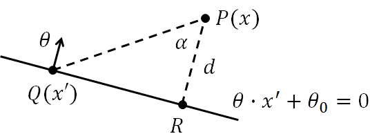
Since $d$ is the smallest possible distance, the vector $\overrightarrow{RP}$ is perpendicular to $\overrightarrow{QR}$ and so the points $PQR$ form a right-angled triangle. The distance $d$ can then be expressed using basic trigonometry,

$$d = \norm{\overrightarrow{RP}} = \norm{\overrightarrow{QP}} \textrm{ cos }\alpha.$$

We also know the angle $\alpha$ is related to $\overrightarrow{QP}$ and $\theta$ by the dot product,

$$ \theta \cdot \overrightarrow{QP} = \norm{\theta} \norm{\overrightarrow{QP}} \textrm{ cos }\alpha .$$

Consolidating these two equations, together with the fact that $\overrightarrow{QP} = x - x',$ yields the final expression for the signed distance,

$$d_s(x) = \frac{ \theta \cdot \overrightarrow{QP} }{\norm{ \theta} } = \frac{ \theta \cdot x - \theta \cdot x' }{\norm{ \theta} } = \frac{ \theta \cdot x + \theta_0 }{\norm{ \theta} }. $$

Signed and unsigned distance

What does it mean for $d$ to be signed? As a quick illustration, consider how a hypothetical classifier might deal with some positive training examples (Fig. 4). We can see that the points “deepest” within the positive region, $x_1$ and $x_2$, are sitting some positive distance from the decision boundary because $\theta \cdot x + \theta_0$ is positive for each point.

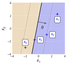
The example $x_2$ is sitting right on the positive margin boundary. Since any point on the positive margin boundary satisfies $\theta \cdot x + \theta_0 = 1$, this means

$$d_s(x_2) = \frac{\theta \cdot x_2 + \theta_0}{\norm{\theta}} = \frac{1}{\norm{\theta}}.$$

We can also see that $x_3$ sits right on the decision boundary, and so

$$d_s(x_3) = 0.$$

What about $x_4$? The dot product of $\theta$ and $x_4$ will be negative, as will be the distance. We know that its distance must be something between zero and $-1/\norm{\theta},$ the signed distance to the negative margin boundary.

We can modify the signed distance slightly to form an expression for the unsigned distance of a training example from the decision boundary by using the example’s label,

$$d(x^{(i)}) = \frac{y^{(i)} ( \theta \cdot x^{(i)} + \theta_0 )}{\norm{\theta}}.$$

It’s time to put all the pieces together.

Learning as optimization

There has been a lot of ground covered since we first brought up the idea of reframing the learning process as an optimization problem. To recap, there are two competing priorities:

• achieving high training set classification accuracy, and
• obtaining large classifier margins.

We are going to formulate an objective function $J$ that incorporates these priorities as two separate components: (a) the average loss, and (b) the regularization component. The idea is then to find the classifier parameters $\theta$ and $\theta_0$ that minimize $J,$ where

$$ J(\theta, \theta_0) = \textrm{average loss} + \lambda \cdot \textrm{regularization}.$$

That lambda parameter $\lambda$ is the regularization term. This is an important parameter that we will soon discuss, but for now, think of it as a dial that we can tweak to balance our two priorities. Let’s now talk about the first component.

Average loss

The average loss component (oddly enough!) makes use of a loss function. The goal of a loss function is to quantify the error of a prediction. You have already seen the 0-1 loss function $f(z^{(i)}, y^{(i)}) = [\![ z^{(i)} \neq y^{(i)} ]\!],$ which takes the value 1 when the prediction $z^{(i)}$ doesn’t match the example label $y^{(i)}$, and zero otherwise.

Another common loss function is the hinge loss function,

$$\textrm{Loss}_h(z) = \begin{cases} 1-z & \text{if $z<1$} \\
0 & \text{otherwise} \end{cases}$$

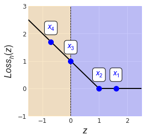
Let’s use the hinge loss function on our (positive) training examples from the last figure. Below we have a plot of the hinge loss function, with the loss of each example overlaid as a blue dot (Fig. 5). Points $x_1$ and $x_2$ incur zero loss, since $z^{(i)} = y^{(i)} (\theta \cdot x^{(i)} + \theta_0) \geq 1$ for both examples. The point $x_3$, sitting on the decision boundary, incurs an agreement value $z^{(3)} = 0$, which gets mapped to $\textrm{Loss}_h(z^{(3)}) = 1 - z^{(3)} = 1.$

We can see that once a point starts to invade its corresponding margin boundary (located at $z=1$ for the positive label), the hinge loss increases linearly as a function of distance.

Using this loss function, the average loss can now be written as

$$\textrm{average loss} = \frac{1}{N} \sum_{i=1}^{N}\textrm{Loss}_h(y^{(i)} ( \theta \cdot x^{(i)} + \theta_0 )).$$

Regularization

At this stage you may have a vague idea that large margin classifiers are a good thing, and that regularization is supposed to help find such classifiers. We will expand on these ideas in this section. The topic of regularization is definitely worth more coverage, since it is critical in helping us avoid the dreaded problem of overfitting.

Models that suffer from overfitting are in a sense, too smart for their own good. Overfit models are too familiar with the training data, contorting themselves to minimize training errors at the expense of being useful for general application.

We will illustrate this problem with some synthetic data: twenty points from a quadratic function, corrupted by some noise. Now let’s fit three different polynomials to this data:

• a linear function,
• a quadratic function (i.e., a proper fit), and
• a 10th-order polynomial.

The overfit model has some issues. It is overly complex for the data: while the average error (or loss) across the training data might be quite low, it is completely useless beyond the limited range of our training data. The linear fit faces the same problem but for the opposite reason: it is too simple to capture the underlying signal.

In the context of our optimization problem, classification accuracy for the training set is improved by minimizing the average loss component. How do we maximize the classifier margins? To do this, we need to minimize $\norm{\theta}$. This is the same task as minimizing $\norm{\theta}^2$. By convention, the regularization component is specified as

$$\textrm{regularization} = \frac{1}{2} \norm{\theta}^2.$$

The objective function

We are finally ready to look at the objective function in all its glory, the function that we are going to minimize to discover the parameters $\{\theta,\theta_0\}$ of our classifier:

$$J(\theta,\theta_0) = \underbrace{\frac{1}{N} \sum_{i=1}^{N}\textrm{Loss}(y^{(i)} ( \theta \cdot x^{(i)} + \theta_0 ))}_{\textrm{average loss}} + \underbrace{ \vphantom{ \sum_{1}^{2} } \frac{\lambda}{2}\norm{\theta}^2.}_{\textrm{regularization}}$$

Within the framework of our optimization problem, we need to strike the right balance between model complexity (minimizing training loss) and model utility (maximizing classifier margins), which is done by finding a good value of $\lambda$.

Before we discuss how to minimize the objective function, it is worth taking a quick detour to talk about what it really means to find a “good” value of $\lambda$.

Bias-variance trade-off

To get a feel for what we are trying to achieve here, let’s frame our discussion around the idea of model “complexity”, $C = \frac{1}{\lambda}$. That makes the objective function look like this:

$$J(\theta,\theta_0) = \frac{1}{N} \sum_{i=1}^{N}\textrm{Loss}(y^{(i)} ( \theta \cdot x^{(i)} + \theta_0 )) + \frac{1}{2C}\norm{\theta}^2.$$

As we increase the model complexity, the regularization component becomes less influential, with more importance placed on minimizing the training error. A model that is too complex (like that tenth-order polynomial from the last figure) will be highly sensitive to the training data – if trained on another training set, the resulting model parameters and its corresponding predictions are likely to be very different. Such a model is said to exhibit high variance (Fig. 7, orange shading).

It is also possible to use a model that is too simple, as you have seen earlier. Notice how smaller values of $C$ place more importance on finding large margin classifiers. An underfit model does not produce accurate predictions, indicating a large bias (Fig. 7, blue shading). You can think of bias as the error inherent to your model. For example, there is a hard limit on how well you can fit a linear function to quadratic-order training data (Fig. 6).

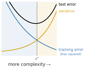
There is one more item of interest here: the test error (Fig. 7, black curve), which is comprised of the model bias and variance. If we can minimize the test error¹, we could then find $C^{\ast}$, the optimal level of complexity that achieves low bias (high prediction accuracy on the test set) and low variance (model parameters that are not sensitive to the choice of training data). The balance between these two priorities is known as the bias-variance trade-off.

Gradient descent

Let’s return to our original discussion. The goal is to find the classifier parameters $\{\theta,\theta_0\}$ by minimizing $J$, the objective function. We will now introduce gradient descent, a well-known iterative algorithm for finding these parameters.

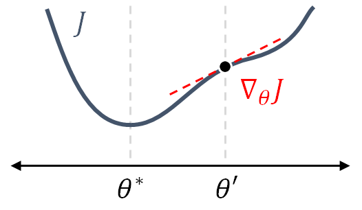
To start with, we will look at what happens in a single iteration of the algorithm, for a single parameter $\theta$ and its associated objective function $J(\theta)$ (Fig. 8). The algorithm starts at some point $\theta_k = \theta'$, located to the right of the ideal value $\theta^*$. Next, the slope (or gradient) $\nabla_{\theta} J = \frac{\partial J}{\partial \theta}$ is evaluated at $\theta_k$. Finally, the algorithm computes $\theta_{k+1}$ by taking a step in the opposite direction of the slope, such that

$$\theta_{k+1} = \theta_{k} - \eta \cdot [\nabla_{\theta} J] _{\theta_k},$$

where the learning rate $\eta$ determines the size of the step. With successive iterations, the parameter gets closer and closer to $\theta^{\ast}$, for which $J(\theta^\ast)$ is a (local) minimum.

The same principles apply in higher dimensions. If we are trying to optimize two parameters $(x, y)$, then both parameters are updated simultaneously using the partial derivatives of $J,$ evaluated at the current parameter values $(x_k, y_k)$.

$$\begin{align*} \begin{bmatrix} x_{k+1}\\
y_{k+1}\\
\end{bmatrix} &= \begin{bmatrix} x_k\\
y_k\\
\end{bmatrix} - \eta \begin{bmatrix} \frac{\partial J}{\partial x}\\
\frac{\partial J}{\partial y}\\
\end{bmatrix}_{(x_k,y_k)} \end{align*}$$

How do we actually compute the gradient? That depends on which loss function is being used. For now we will show the general expression for the gradient, leaving out the offset parameter for cleaner notation, but either way, we can see that the gradient is just a sum of functions.

$$\begin{align*} \nabla_{\theta} J(\theta) &= \nabla_{\theta} \left [ \frac{1}{N} \sum_{i=1}^{N}\textrm{Loss}(y^{(i)} \theta \cdot x^{(i)} ) \right ] + \nabla_{\theta} \left [ \frac{\lambda}{2}\norm{\theta}^2 \right ]\\
&= \frac{1}{N} \sum_{i=1}^{N} \nabla_{\theta} \left [ \textrm{Loss}(y^{(i)} \theta \cdot x^{(i)} ) \right ] + \lambda \theta \end{align*}$$

Note that we need to iterate over the entire dataset for each gradient update, which can be resource-intensive and oftentimes inconvenient. It is largely for these reasons that we consider an alternative algorithm, one that has become a mainstay in the modern ML practitioner’s toolbox.

Stochastic gradient descent

The basic idea behind stochastic gradient descent (SGD) is to approximate the objective function gradient $\nabla_{\theta} J(\theta)$ using a randomly selected sample $(x^{(i)}, y^{(i)})$ from the full dataset. The expression for the gradient then becomes

$$\begin{align*} \nabla_{\theta} J_i(\theta) &= \nabla_{\theta} \textrm{Loss}(y^{(i)} \theta \cdot x^{(i)} ) + \lambda \theta \end{align*}.$$

Let’s assume that we’re dealing with hinge loss, whose derivative looks like this:

$$ \nabla_z \textrm{Loss}_h(z) = \begin{cases} -1 & \text{if $z<1$} \\
0 & \text{otherwise} \end{cases}$$

The objective function gradient for the $i$-th example now takes the form

$$\begin{align*} \nabla_{\theta} J_i(\theta) &= \begin{cases} -y^{(i)} x^{(i)} + \lambda \theta & \text{if loss > 0}\\
\lambda \theta & \text{if loss = 0} \end{cases} \end{align*}$$

As you might guess, this “cheap” gradient tends to increase the number of iterations needed to converge on the optimized model parameters. On the other hand, each iteration can be computed much more rapidly, with especially good performance made possible on high-dimensional datasets.

Summary

The objective function is an important construct that lets us reframe machine learning problems as optimization problems, which can be solved with the help of some calculus. We have discussed a handful of important considerations that apply to most (if not all) ML problems, but there is of course so much more to learn. For those wondering where to go from here, my suggestion would be to read up about different types of regularization and how they can be used to achieve different outcomes (e.g., lasso regularization can be used to eliminate unhelpful predictors in a regression model).